李宏毅教授2021年机器学习课程的作业,详见ML 2021 Spring
感觉NTU学生的英语都很好啊hh,所以这也是本人第一次练习使用双语书写注释及内容
Homework 1: COVID-19 Cases Prediction (Regression)
Simple Baseline
只要跑通助教的代码就可以,经注释后的代码如下。
Download Data
If the Google drive links are dead, you can download data from kaggle, and upload data manually to the workspace.
1 | tr_path = 'covid.train.csv' # path to training data |
1 | /usr/local/lib/python3.7/dist-packages/gdown/cli.py:131: FutureWarning: Option `--id` was deprecated in version 4.3.1 and will be removed in 5.0. You don't need to pass it anymore to use a file ID. |
Import Some Packages
1 | # PyTorch |
Some Utilities
You do not need to modify this part.
1 | def get_device(): |
Preprocess
We have three kinds of datasets:
train: for trainingdev: for validationtest: for testing (w/o target value)
Dataset
The COVID19Dataset below does:
- read
.csvfiles - extract features
- split
covid.train.csvinto train/dev sets - normalize features
Finishing TODO below might make you pass medium baseline.
1 | class COVID19Dataset(Dataset): |
DataLoader
A DataLoader loads data from a given Dataset into batches.
1 | def prep_dataloader(path, mode, batch_size, n_jobs=0, target_only=False): |
Deep Neural Network
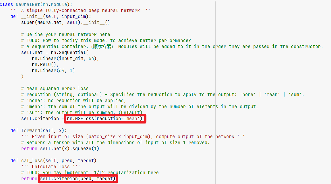
NeuralNet is an nn.Module designed for regression.
The DNN consists of 2 fully-connected layers with ReLU activation.
This module also included a function cal_loss for calculating loss.
1 | class NeuralNet(nn.Module): |
Train/Dev/Test
Training
1 | def train(tr_set, dv_set, model, config, device): |
Validation
1 | def dev(dv_set, model, device): |
Testing
1 | def test(tt_set, model, device): |
Setup Hyper-parameters
config contains hyper-parameters for training and the path to save your model.
1 | device = get_device() # get the current available device ('cpu' or 'cuda') |
Load data and model
1 | tr_set = prep_dataloader(tr_path, 'train', config['batch_size'], target_only=target_only) |
1 | Finished reading the train set of COVID19 Dataset (2430 samples found, each dim = 93) |
1 | model = NeuralNet(tr_set.dataset.dim).to(device) # Construct model and move to device |
Start Training!
1 | model_loss, model_loss_record = train(tr_set, dv_set, model, config, device) |
Saving model (epoch =    1, loss =  78.8524)
Saving model (epoch =    2, loss =  37.6170)
Saving model (epoch =    3, loss =  26.1203)
Saving model (epoch =    4, loss =  16.1862)
Saving model (epoch =    5, loss =  9.7153)
Saving model (epoch =    6, loss =  6.3701)
Saving model (epoch =    7, loss =  5.1802)
Saving model (epoch =    8, loss =  4.4255)
Saving model (epoch =    9, loss =  3.8009)
Saving model (epoch =   10, loss =  3.3691)
Saving model (epoch =   11, loss =  3.0943)
Saving model (epoch =   12, loss =  2.8176)
Saving model (epoch =   13, loss =  2.6274)
Saving model (epoch =   14, loss =  2.4542)
Saving model (epoch =   15, loss =  2.3012)
Saving model (epoch =   16, loss =  2.1766)
Saving model (epoch =   17, loss =  2.0641)
Saving model (epoch =   18, loss =  1.9399)
Saving model (epoch =   19, loss =  1.8978)
Saving model (epoch =   20, loss =  1.7950)
Saving model (epoch =   21, loss =  1.7164)
Saving model (epoch =   22, loss =  1.6455)
Saving model (epoch =   23, loss =  1.5912)
Saving model (epoch =   24, loss =  1.5599)
Saving model (epoch =   25, loss =  1.5197)
Saving model (epoch =   26, loss =  1.4698)
Saving model (epoch =   27, loss =  1.4189)
Saving model (epoch =   28, loss =  1.3992)
Saving model (epoch =   29, loss =  1.3696)
Saving model (epoch =   30, loss =  1.3442)
Saving model (epoch =   31, loss =  1.3231)
Saving model (epoch =   32, loss =  1.2834)
Saving model (epoch =   33, loss =  1.2804)
Saving model (epoch =   34, loss =  1.2471)
Saving model (epoch =   36, loss =  1.2414)
Saving model (epoch =   37, loss =  1.2138)
Saving model (epoch =   38, loss =  1.2083)
Saving model (epoch =   41, loss =  1.1591)
Saving model (epoch =   42, loss =  1.1484)
Saving model (epoch =   44, loss =  1.1209)
Saving model (epoch =   47, loss =  1.1122)
Saving model (epoch =   48, loss =  1.0937)
Saving model (epoch =   50, loss =  1.0842)
Saving model (epoch =   53, loss =  1.0655)
Saving model (epoch =   54, loss =  1.0613)
Saving model (epoch =   57, loss =  1.0524)
Saving model (epoch =   58, loss =  1.0394)
Saving model (epoch =   60, loss =  1.0267)
Saving model (epoch =   63, loss =  1.0248)
Saving model (epoch =   66, loss =  1.0099)
Saving model (epoch =   70, loss =  0.9829)
Saving model (epoch =   72, loss =  0.9817)
Saving model (epoch =   73, loss =  0.9743)
Saving model (epoch =   75, loss =  0.9671)
Saving model (epoch =   78, loss =  0.9643)
Saving model (epoch =   79, loss =  0.9597)
Saving model (epoch =   85, loss =  0.9549)
Saving model (epoch =   86, loss =  0.9535)
Saving model (epoch =   90, loss =  0.9467)
Saving model (epoch =   92, loss =  0.9432)
Saving model (epoch =   93, loss =  0.9231)
Saving model (epoch =   95, loss =  0.9127)
Saving model (epoch =  104, loss =  0.9117)
Saving model (epoch =  107, loss =  0.8994)
Saving model (epoch =  110, loss =  0.8935)
Saving model (epoch =  116, loss =  0.8882)
Saving model (epoch =  124, loss =  0.8872)
Saving model (epoch =  128, loss =  0.8724)
Saving model (epoch =  134, loss =  0.8722)
Saving model (epoch =  139, loss =  0.8677)
Saving model (epoch =  146, loss =  0.8654)
Saving model (epoch =  156, loss =  0.8642)
Saving model (epoch =  159, loss =  0.8528)
Saving model (epoch =  167, loss =  0.8494)
Saving model (epoch =  173, loss =  0.8492)
Saving model (epoch =  176, loss =  0.8461)
Saving model (epoch =  178, loss =  0.8403)
Saving model (epoch =  182, loss =  0.8375)
Saving model (epoch =  199, loss =  0.8295)
Saving model (epoch =  212, loss =  0.8273)
Saving model (epoch =  235, loss =  0.8252)
Saving model (epoch =  238, loss =  0.8233)
Saving model (epoch =  251, loss =  0.8211)
Saving model (epoch =  253, loss =  0.8205)
Saving model (epoch =  258, loss =  0.8175)
Saving model (epoch =  284, loss =  0.8143)
Saving model (epoch =  308, loss =  0.8136)
Saving model (epoch =  312, loss =  0.8075)
Saving model (epoch =  324, loss =  0.8045)
Saving model (epoch =  400, loss =  0.8040)
Saving model (epoch =  404, loss =  0.8010)
Saving model (epoch =  466, loss =  0.7998)
Saving model (epoch =  525, loss =  0.7993)
Saving model (epoch =  561, loss =  0.7945)
Saving model (epoch =  584, loss =  0.7903)
Saving model (epoch =  667, loss =  0.7896)
Saving model (epoch =  717, loss =  0.7823)
Saving model (epoch =  776, loss =  0.7812)
Saving model (epoch =  835, loss =  0.7797)
Saving model (epoch =  866, loss =  0.7771)
Saving model (epoch =  919, loss =  0.7770)
Saving model (epoch =  933, loss =  0.7748)
Saving model (epoch =  965, loss =  0.7705)
Saving model (epoch =  1027, loss =  0.7674)
Saving model (epoch =  1119, loss =  0.7647)
Saving model (epoch =  1140, loss =  0.7643)
Saving model (epoch =  1196, loss =  0.7620)
Saving model (epoch =  1234, loss =  0.7616)
Saving model (epoch =  1243, loss =  0.7582)
Finished training after 1444 epochs
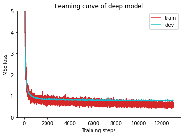
1 | plot_learning_curve(model_loss_record, title='deep model') |
1 | del model # delete model variable |
Testing
The predictions of your model on testing set will be stored at pred.csv.
1 | def save_pred(preds, file): |
Saving results to pred.csv
Medium Baseline
Simple Baseline Code中标注了一些TODO,TA说只要完成这些TODO也许就可以达到Medium Baseline,TODO一共有这些:
- TODO: Using 40 states & 2 tested_positive features (indices = 57 & 75)
- TODO: How to modify this model to achieve better performance?
- TODO: you may implement L1/L2 regularization here
- TODO: How to tune these hyper-parameters to improve your model’s performance?
其中最重要的是TODO1,按TA所说修改即可达到Medium Baseline,即:
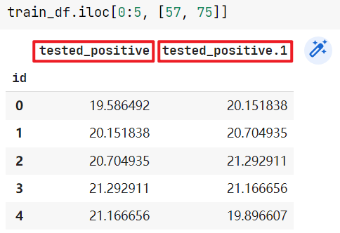
1 | feats = list(range(40)) + [57] + [75] |
查看一下这两列数据,发现列名为tested_positive和tested_positive.1,即第1天阳性和第2天阳性,我们要预测的就是93th列——tested_positive2
Strong Baseline
TA给了以下提示
- Feature selection (what other features are useful?)
- DNN architecture (layers? dimension? activation function?)
- Training (mini-batch? optimizer? learning rate?)
- L2 regularization
- There are some mistakes in the sample code, can you find them?
总的来说就是从三部分优化:1. Data、2. Network Structure、3. Optimization
在本题中最重要的还是Feature selection。
关于1:
可以使用SelectKBest函数,也可以对tested_positive2分析相关性(方法2,还没整理)
1 | import pandas as pd |
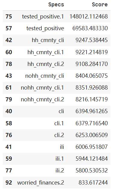
最后一行Score太低,去掉
可以得到改进:
1 | feats = [75, 57, 42, 60, 78, 43, 61, 79, 40, 58, 76, 41, 59, 77] |
关于2:
该作业中“浅的”网络效果更好(Less is More),与后续作业不同,使用如下结构:
1 | self.net = nn.Sequential( |
关于3:
1 | config = { |
关于4:
TA说使用L2正则化,但其实效果提升不大
L1正则化的损失函数
L2正则化的损失函数
1 | def cal_loss(self, pred, target): |
关于5:
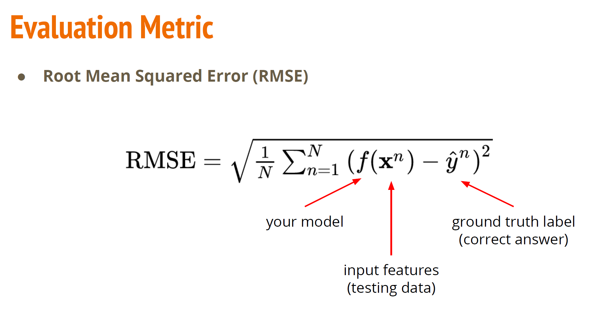
改为
1 | return torch.sqrt(self.criterion(pred, target)) |
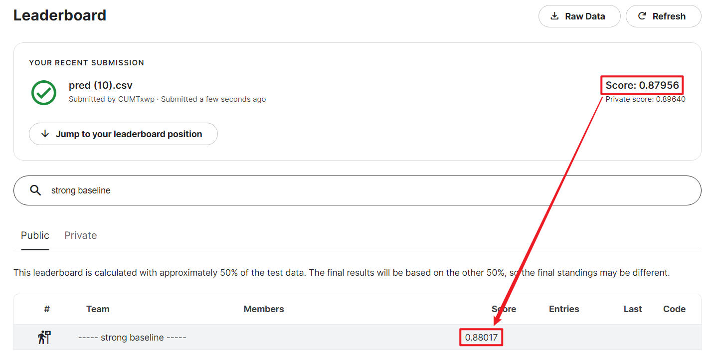
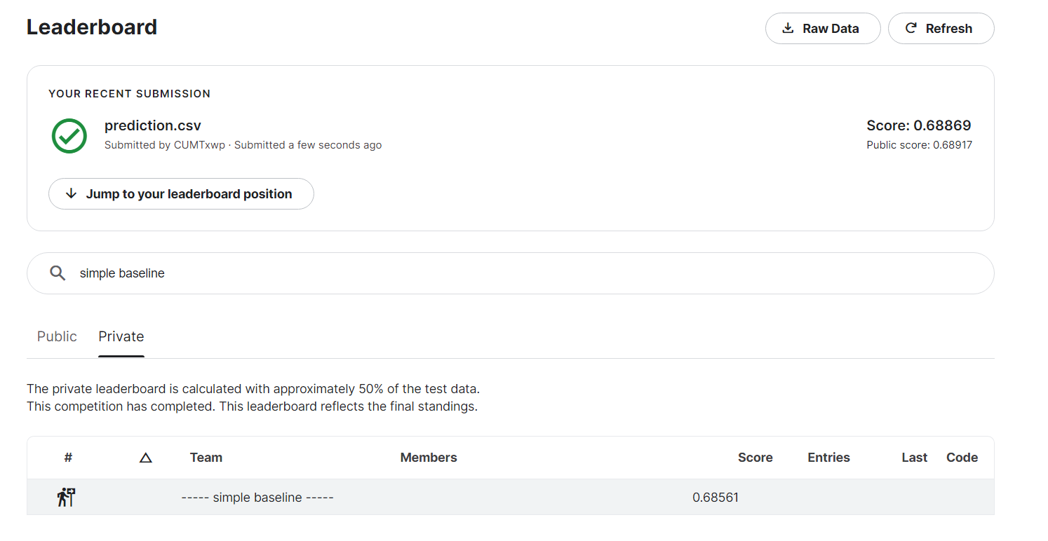
最后过了public的strong baseline,private差0.00x
Homework 2: TIMIT framewise phoneme (classification)
Phoneme Classification - Simple Baseline
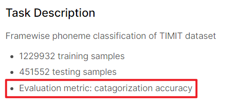
首先可以看到Evaluation metric就是acc,所以越高越好。
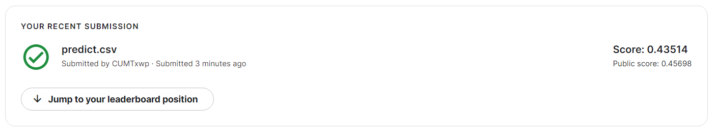
跑通TA’s sample code就可以双过simple baseline
ps:跑一次挺慢的,colab挂上GPU也要15min左右一次。
CODE:
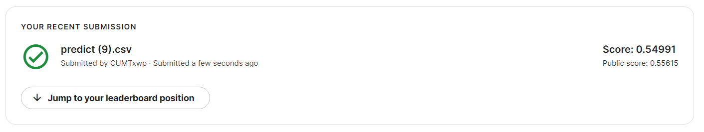
Phoneme Classification - Strong Baseline
TA在PPT里给了一些Hint。
- Model architecture (layers? dimension? activation function?)
- Training (batch size? optimizer? learning rate? epoch?)
- Tips (batch norm? dropout? regularization?)
基本还是Data、Structure、Optimization。
1-百万级数据集,所以VAL_RATIO设为5%
1 | VAL_RATIO = 0.05 |

2-使用RAdam调优
1 | from torch.optim import RAdam |
Hessian Matrix
Homework 3: Convolutional Neural Network - Image Classfication(CNN)
Simple Baseline
直接跑通可以双过simple baseline(需要fix一个好的seed),含注释的原始代码如下:
TA’s Slide: Build a convolutional neural network using labeled images with provided codes.
意思是只要使用给的CNN就可以过simple baseline。
Medium Baseline
TA’s Slide: Improve the performance using labeled images with different model architectures or data augmentations.
TA给了两个方向different model architectures或者data augmentations。
还是在那个范围内:Data、Structure、Optimization。
我们这里尝试一下data augmentations
(好像model architectures要使用resnet?)
增强处:水平反转、旋转、自动增强
1 | from torchvision.transforms.transforms import RandomHorizontalFlip |
然后把原data和增强data拼接起来,这样就有足够的train data了。
1 | train_set1 = DatasetFolder("food-11/training/labeled", loader=lambda x: Image.open(x), extensions="jpg", transform=train_tfm1) |
然后再对learning rate和n_epochs调参调参调参。。。
结果:双过maedium baseline
注1:这里还有一个使用ImageNet的mean和var做标准化的方法,但是我不太会用,加上去效果没有更好。
1 | preprocess = transforms.Compose([ |
注2:关于各种transform方法的实例,详见pytorch教程ILLUSTRATION OF TRANSFORMS
Strong Baseline
TA’s Slide: Improve the performance with additional unlabeled images.
TA将本次作业数据集中的大部分labeled images变成了unlabeled images,这里也是想要让学生练习Semi-supervised Learning(自监督学习)。
那么我们就来试一下Semi-supervised Learning。
首先构建PseudoDataset
1 | class PseudoDataset(Dataset): |
然后修改get_pseudo_labels
1 | def get_pseudo_labels(dataset, model, threshold=0.65): |
在Training中加入semi-supervised learning。
注意两点:
- 当验证集最好精度达到一定值时再开始semi-supervised learning,否则model对unlabel datas的label不准确。
- 为了避免semi-supervised learning影响效率,每semi_turns轮进行一次pseudo。
1 | for epoch in range(n_epochs): |
最后我又调整了transform和CNN architecture,然而这样的效果也不尽人意

最后一条可行的思路是加入Sampler,也就是说新拼接的数据集的dataloader应尽量选取labeled dataset,少选取pseudo dataset。
但是我发现自己再进行下去完全是在做无用功,等把后面的课听完再回来做一做试试,所以目前就到此为止了。
Course中的小知识点
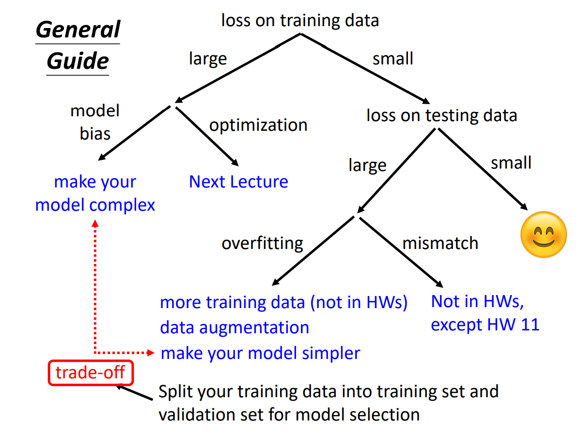
如何降低loss
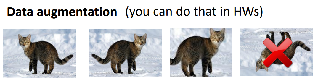
data Augmentation
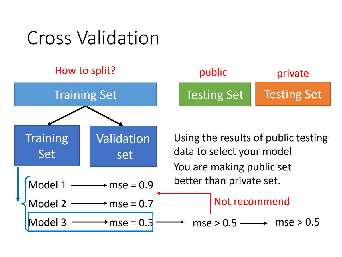
cross validation
避免public testing set和private testing set差距过大
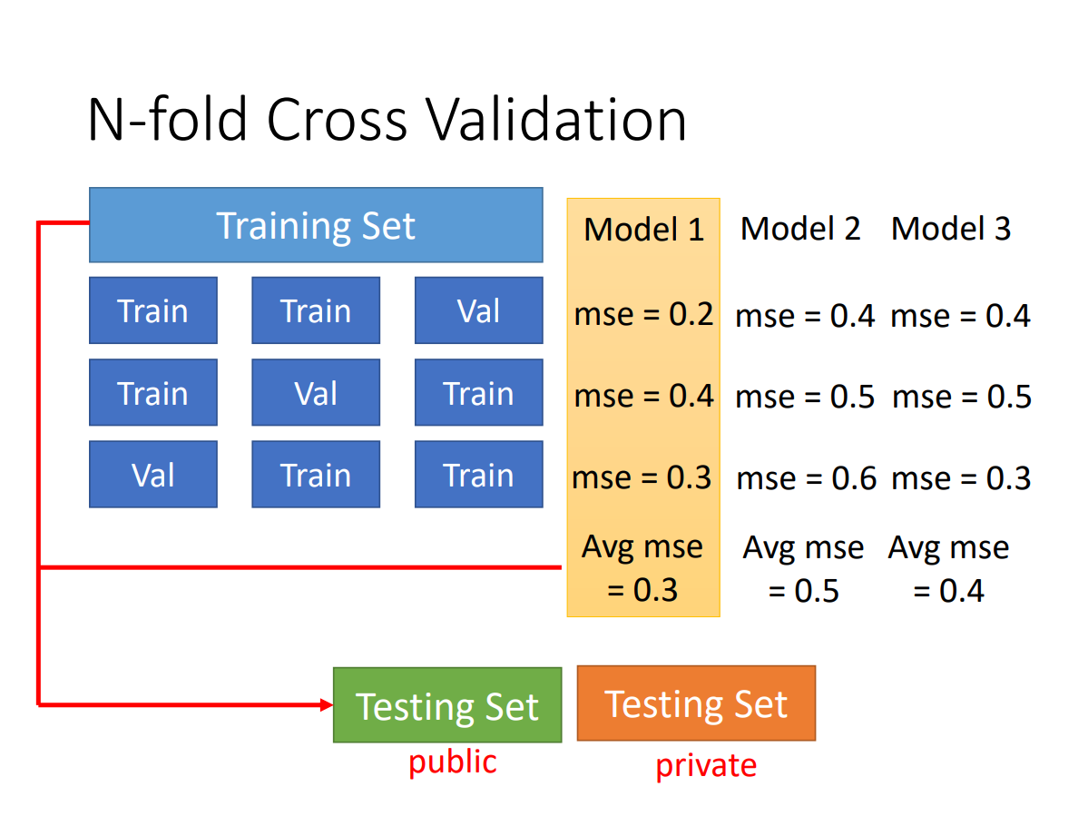
k-fold cross validation
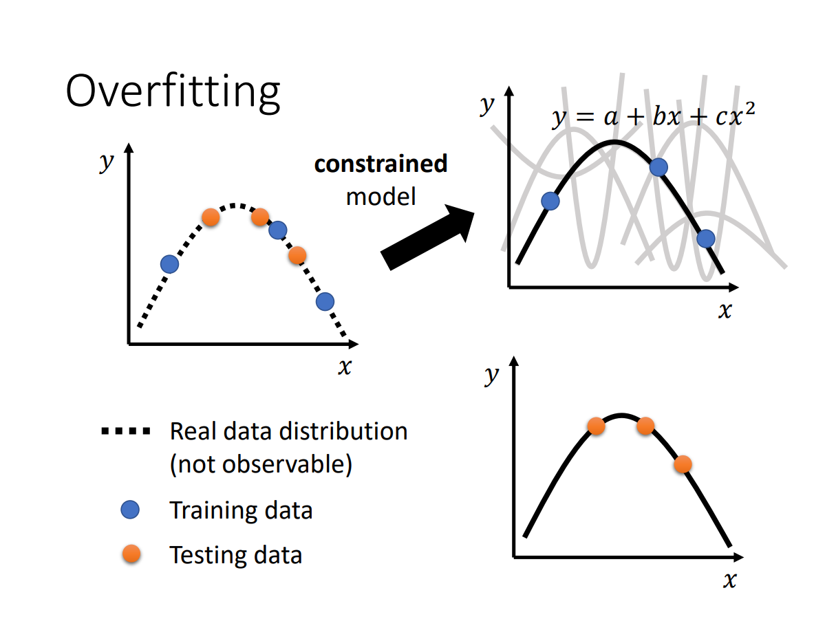
overfitting
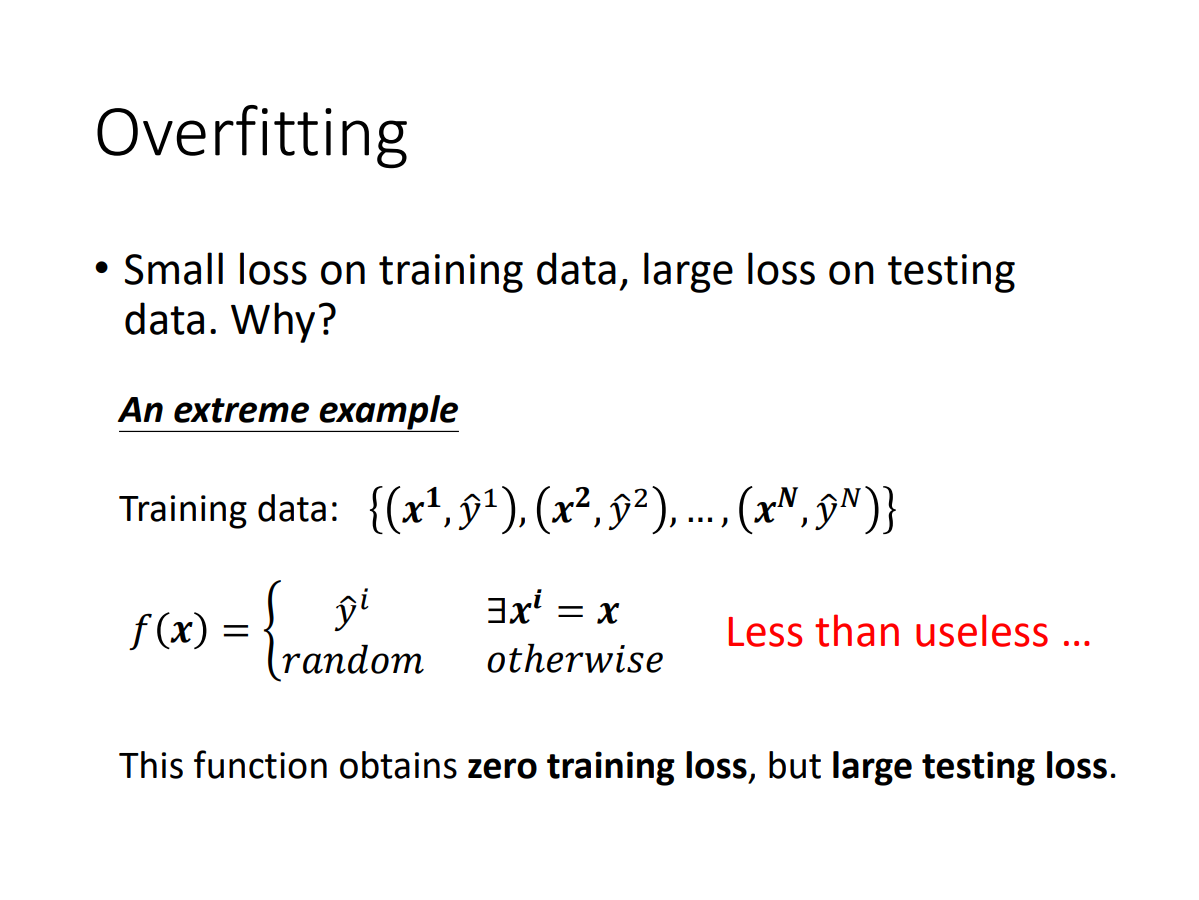
极端的例子:model在训练集上100%准确(loss=0),在测试集上准确度接近0%(loss很大)
原因:
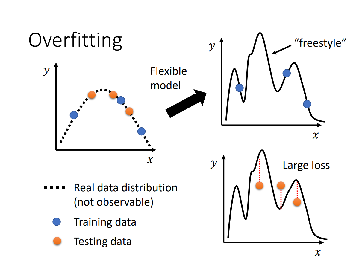
model的flexibility
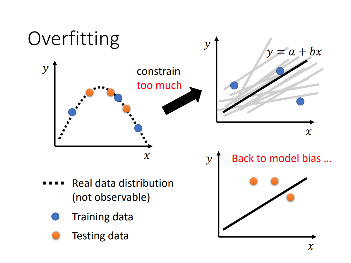
可以通过调整层数来constrain模型,或者增加training data(数据不够?可以Data Augmentation)
但不能constrain过度
mismatch
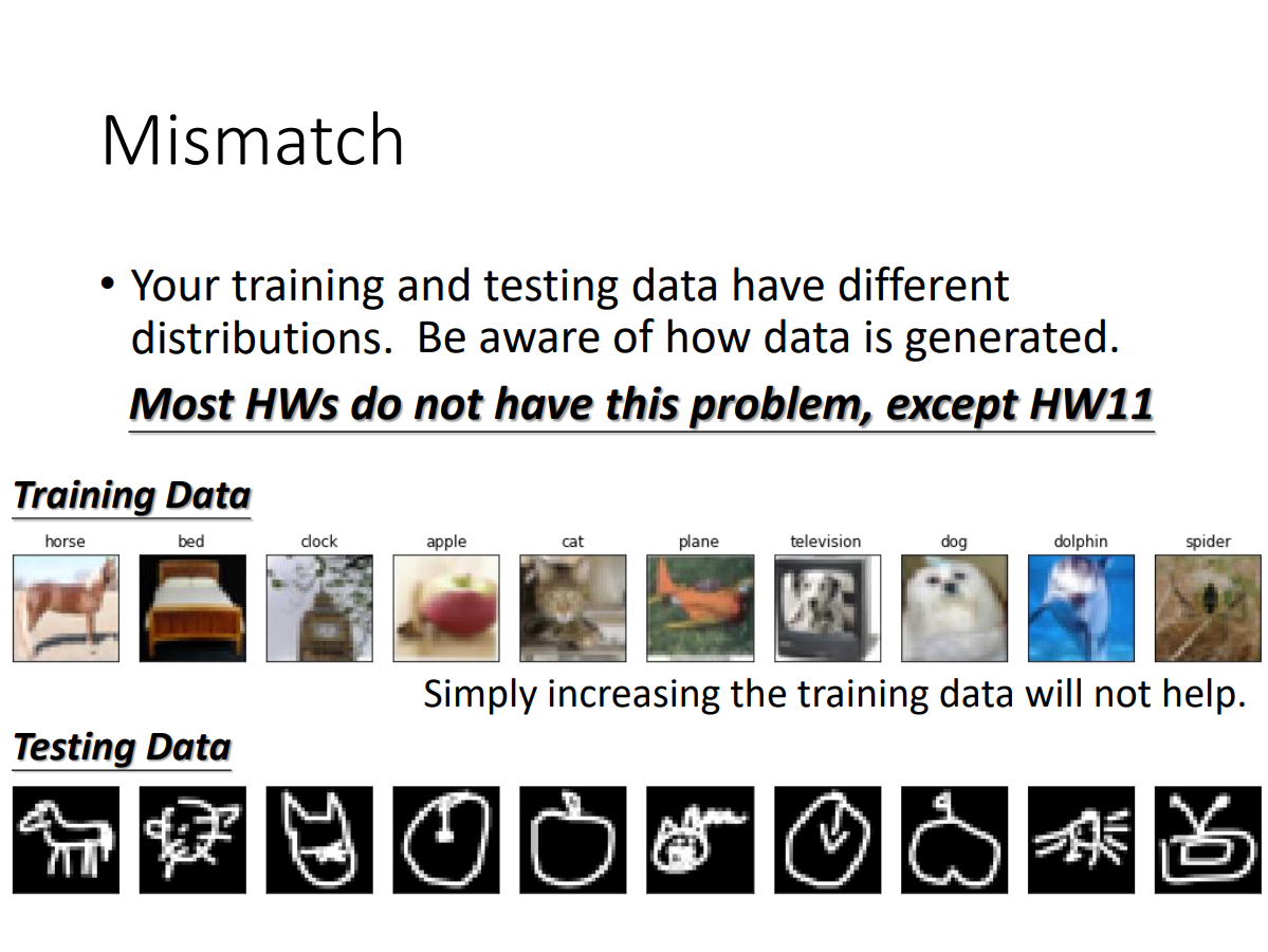
eg.
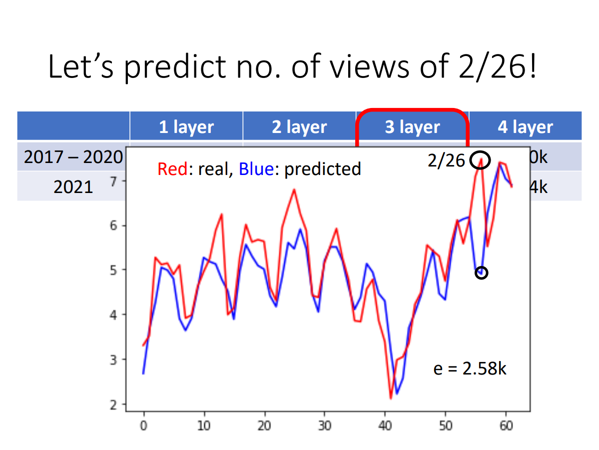
Hung-yi Lee:感谢大家为了让这个模型不准,上周五花了很多力气去点了这个video,所以这一天(2021.2.26)是今年观看人数最多的一天!
(哈哈哈哈笑死我了)
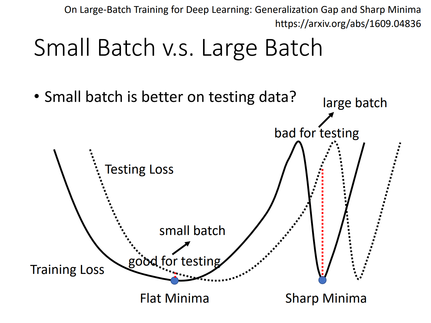
flat minima/sharp minima
好minima和坏minima
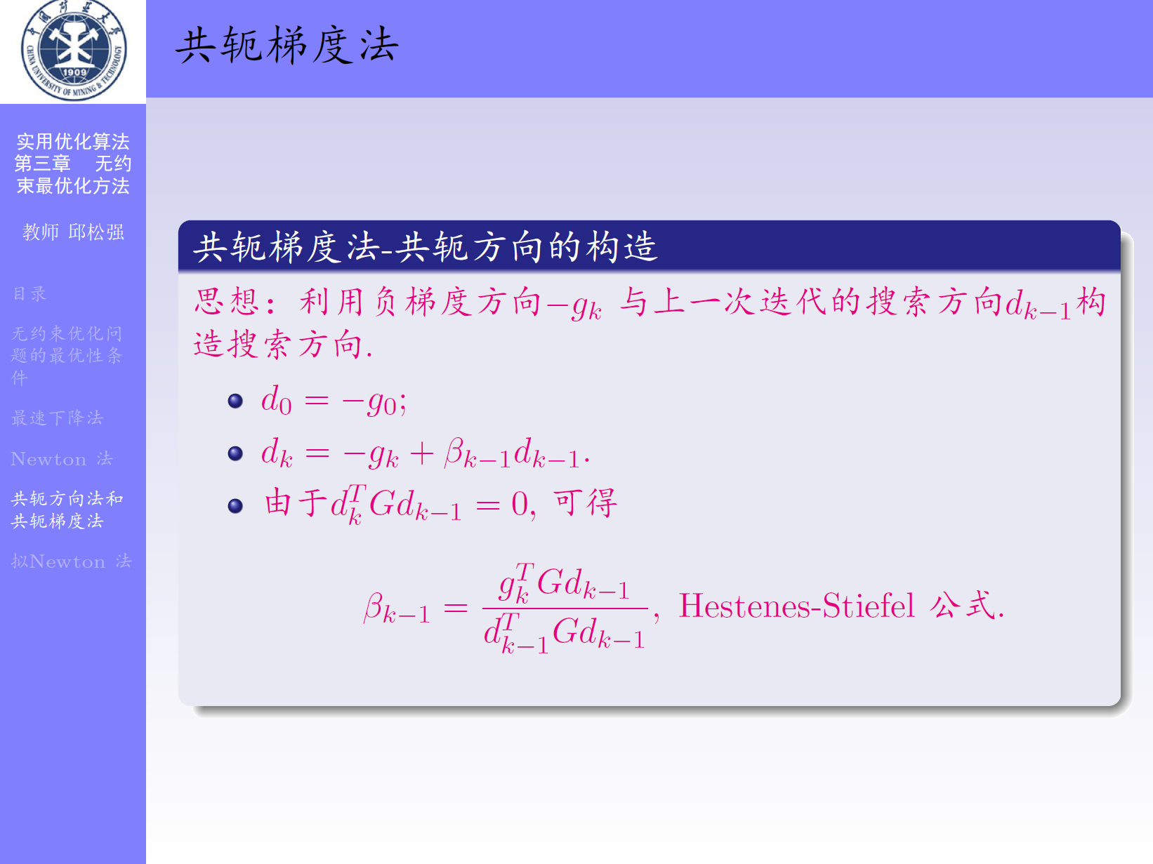
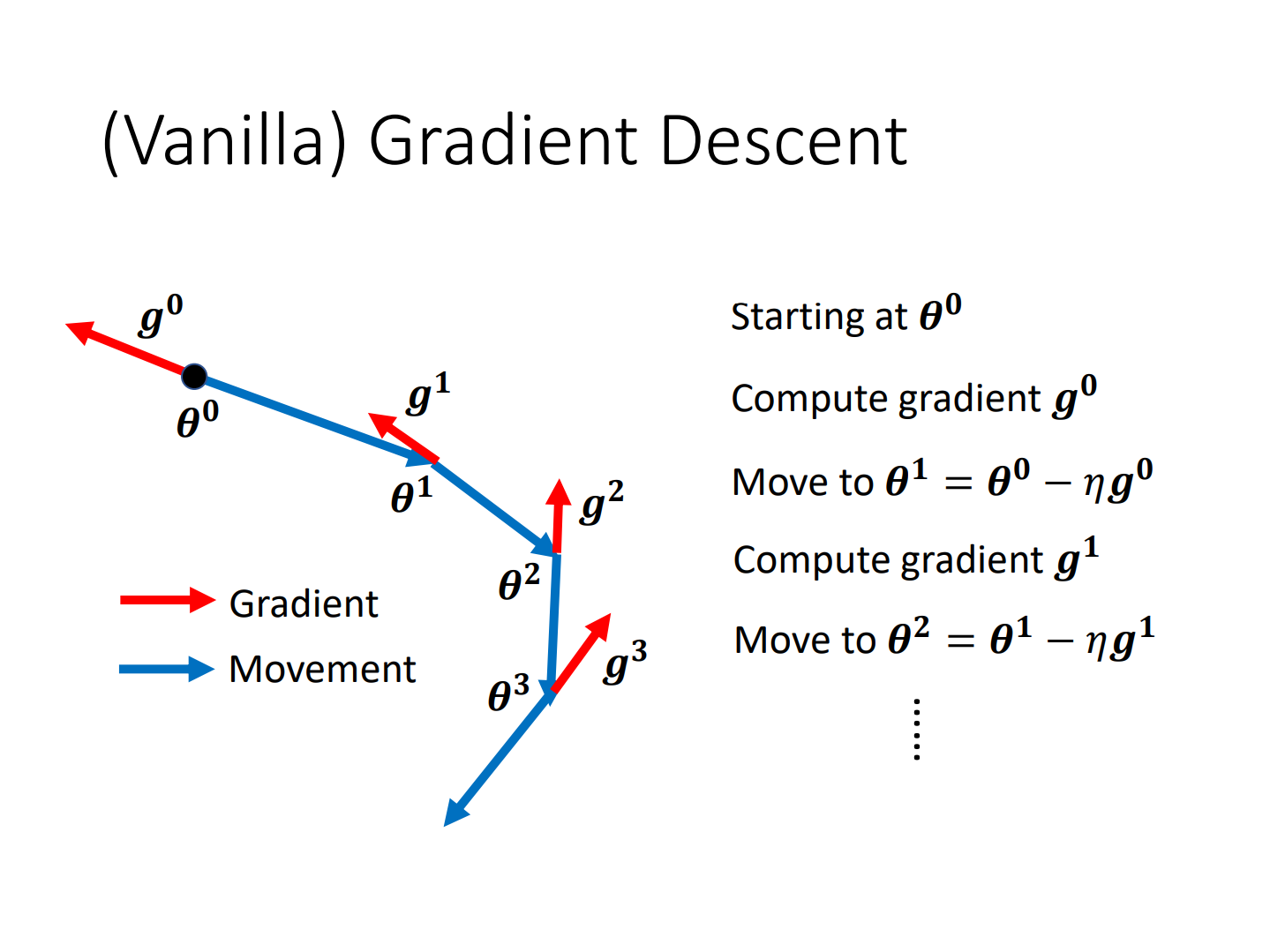
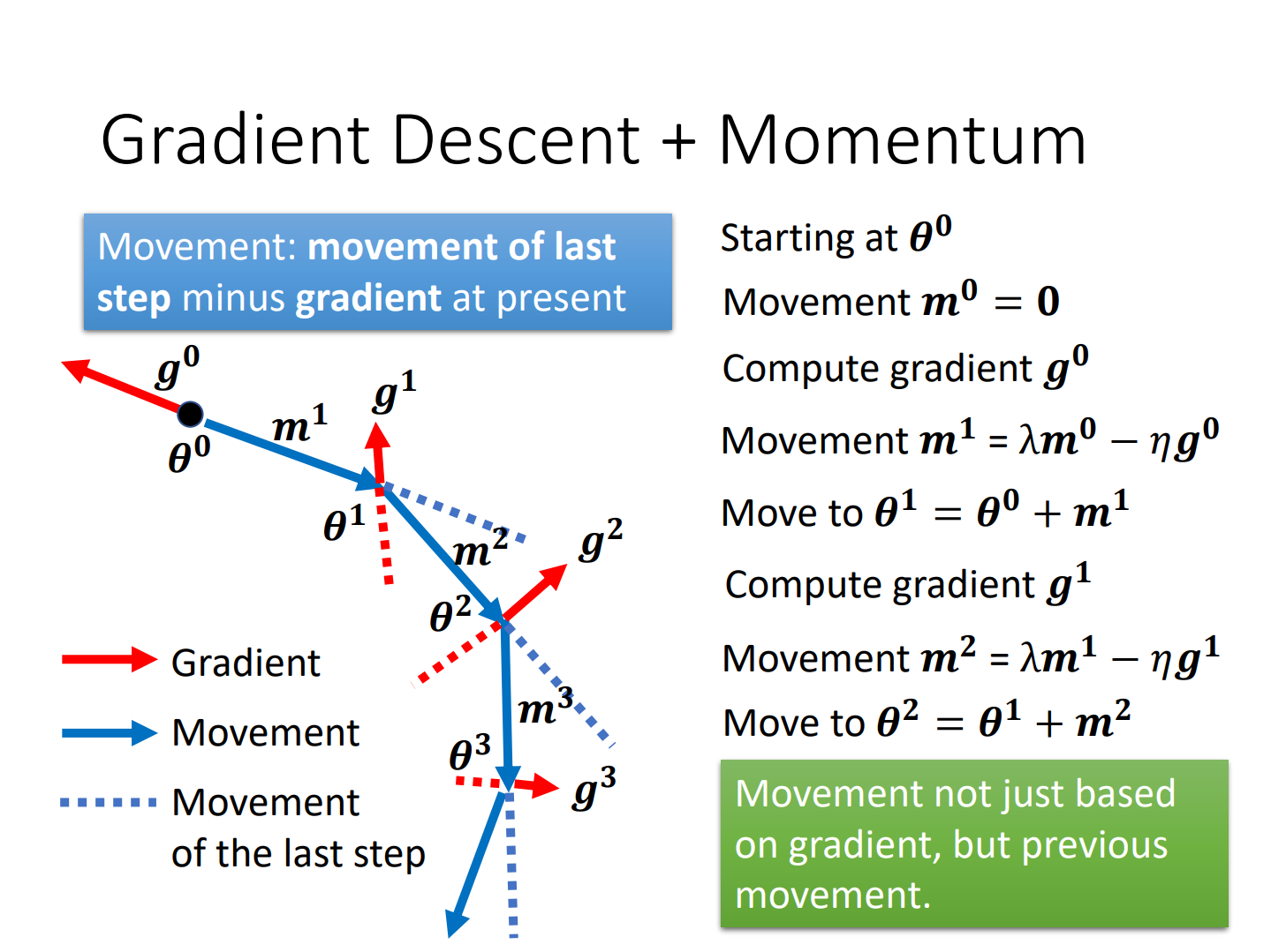
vanilla GD/GD with momentum
总感觉最优化理论学过,但是有点不记得了
很像共轭梯度法!
hylee老师讲的:
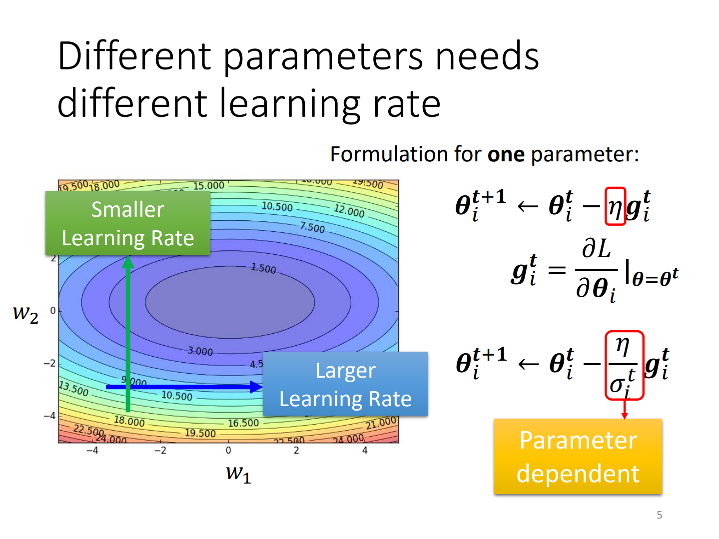
Adaptive Learning Rate(AdaGrad)
Define
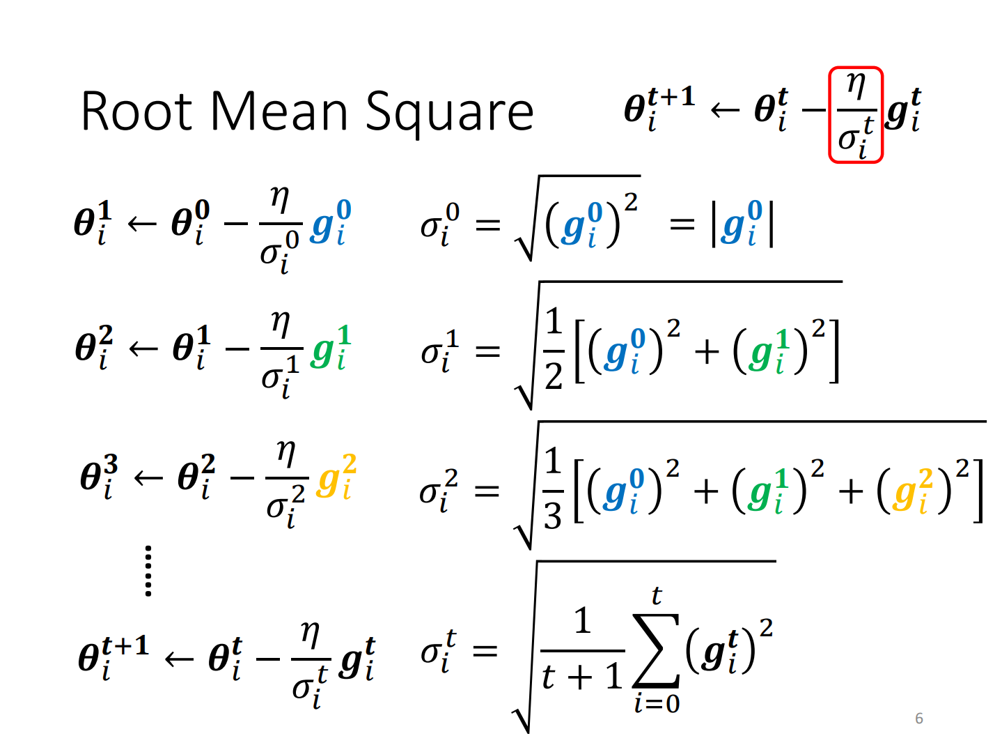
root mean square:均方根
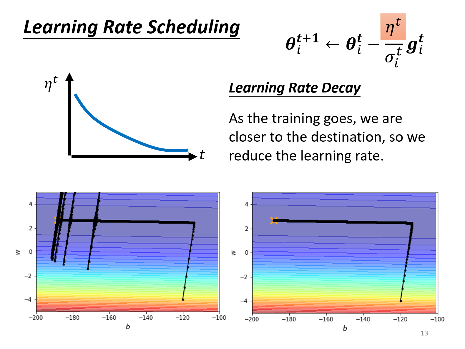
Scheduling
Decay
warmup
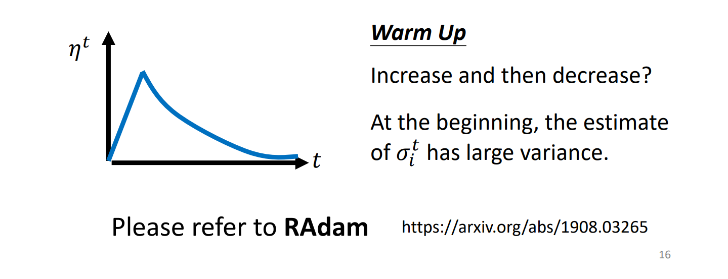
learning rate adapts dynamically(RMSProp)
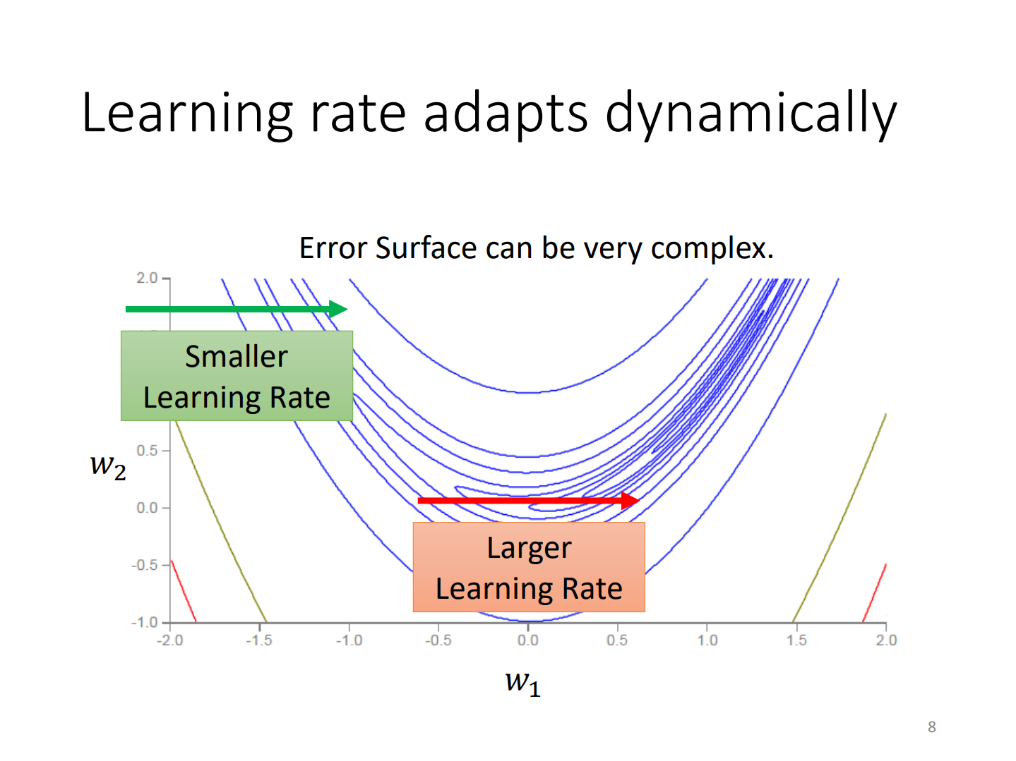
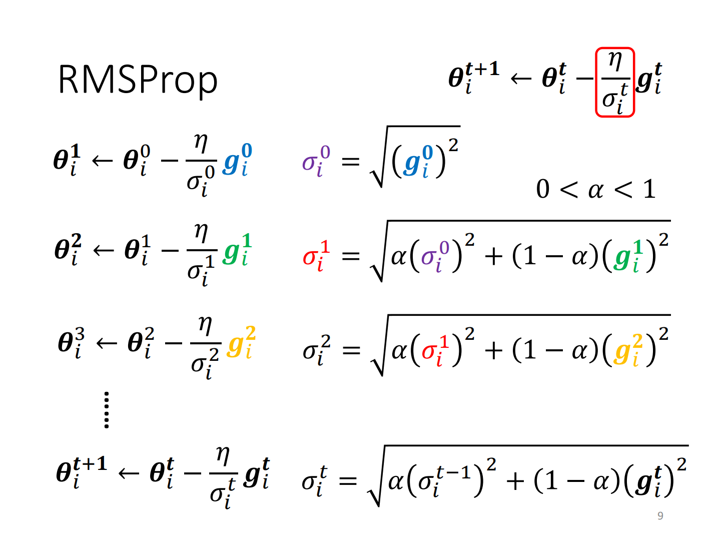
RMSProp:RMS+支点
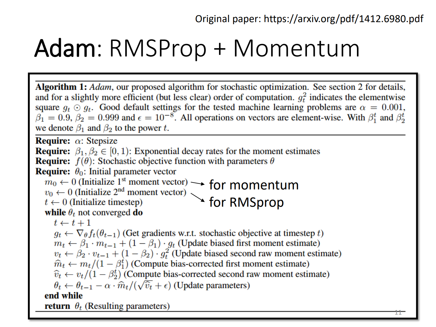
RMSProp + Momentum(Adam)
Cross-entropy
交叉熵
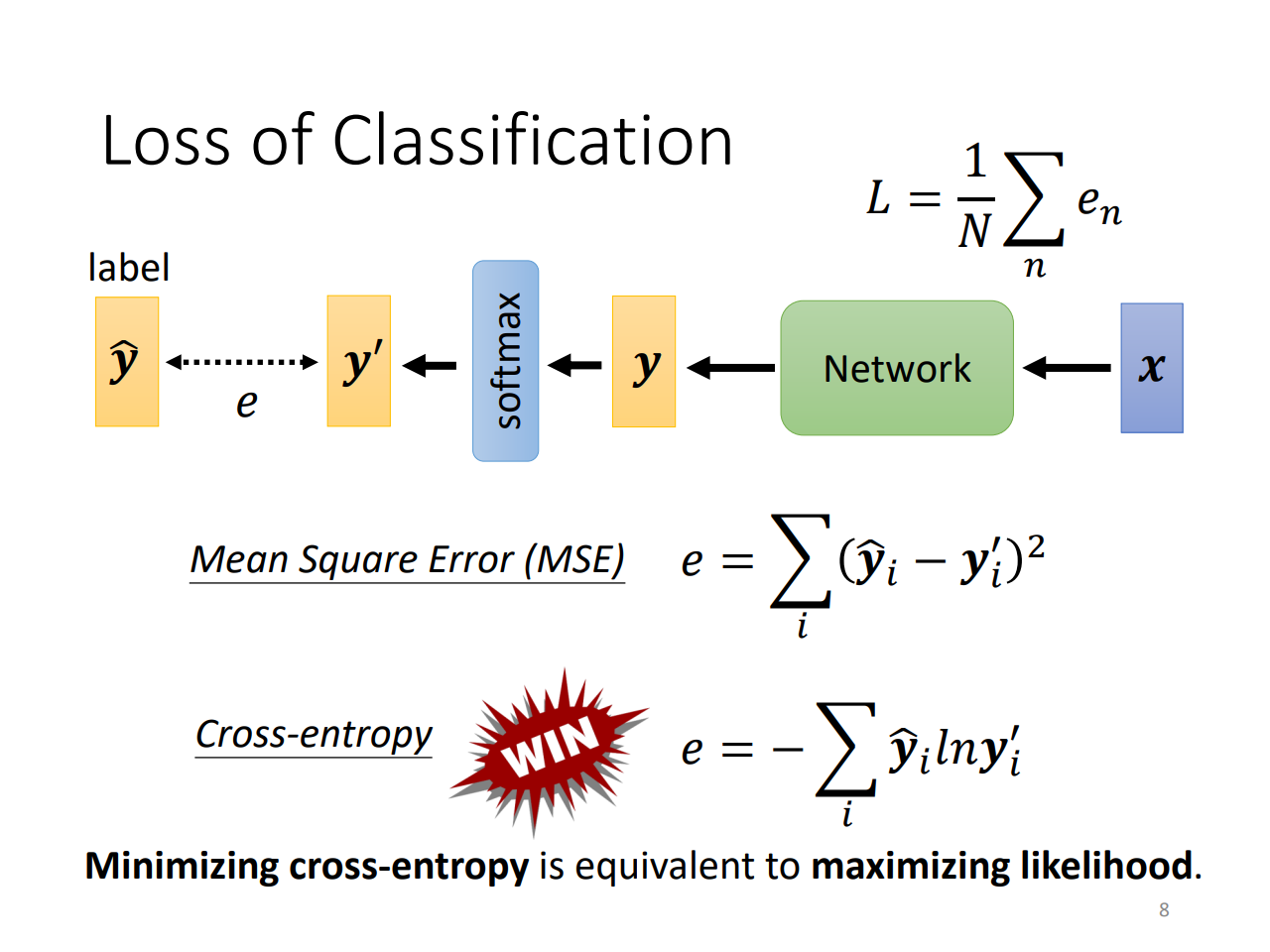
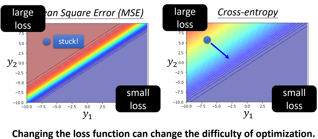
loss function会改变optimization的难度!
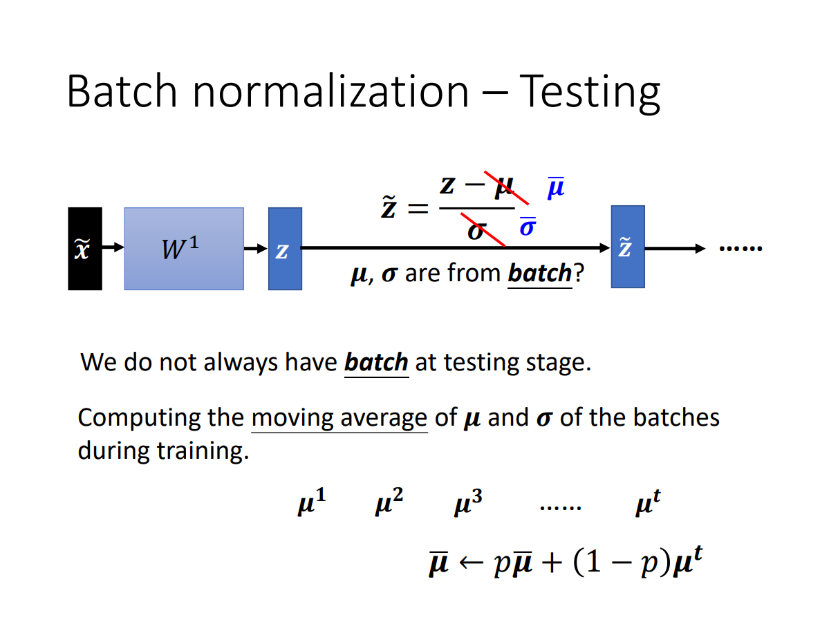
Batch Normalization(BN)
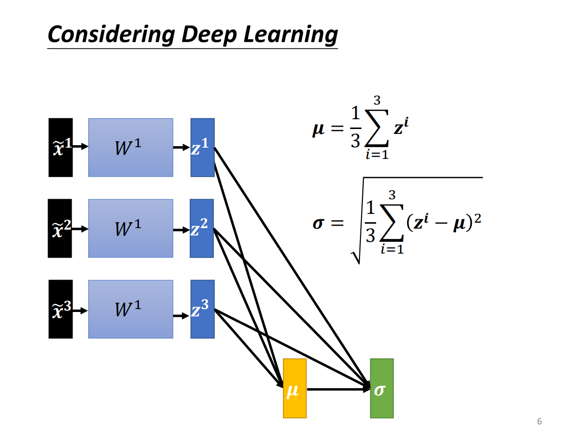
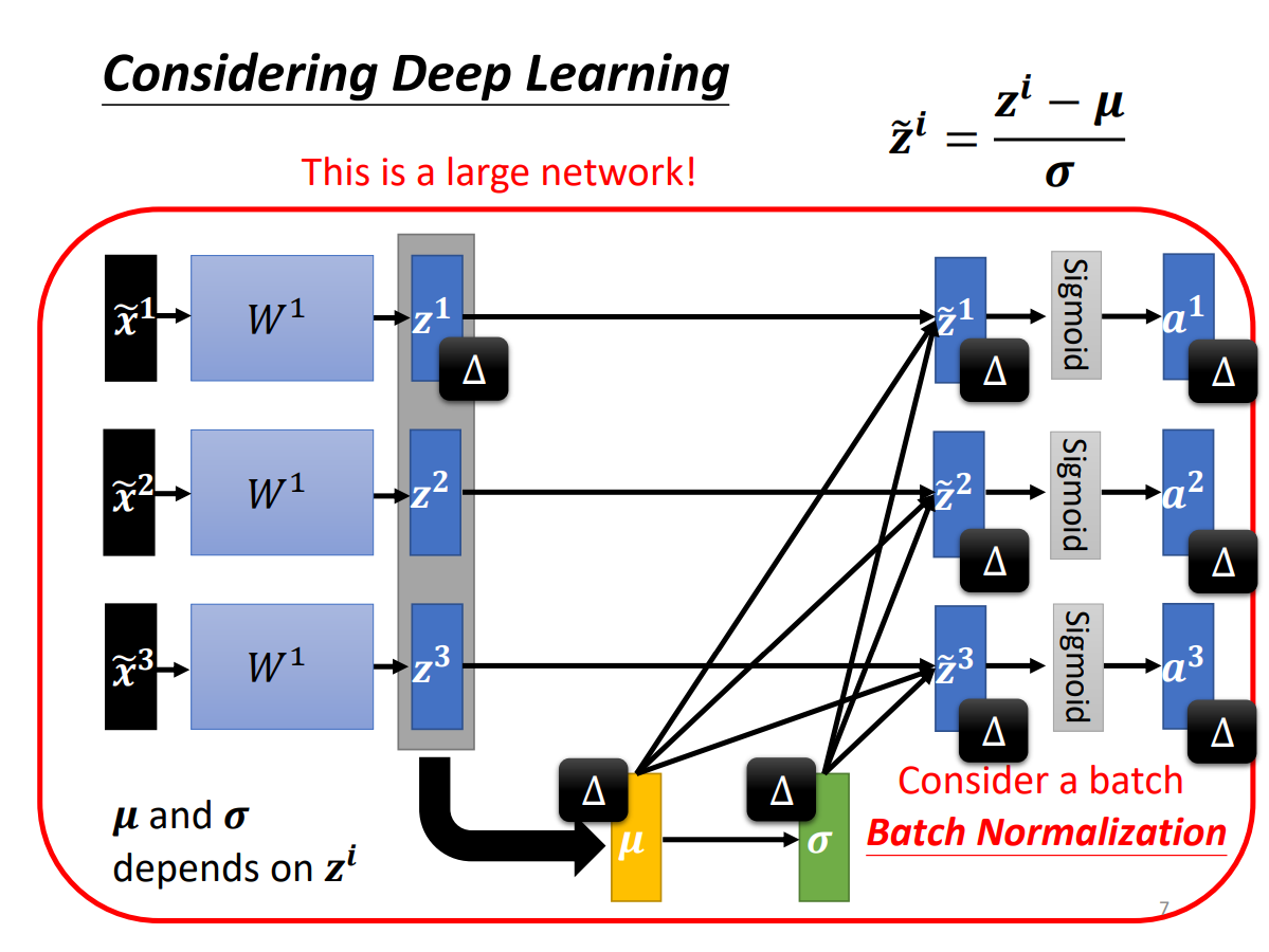
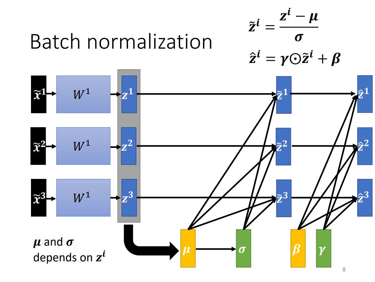
notation
$\hat{y}$:y hat
$e^x$:exponential x
$\sum$:Summation
$y{\prime}$:y prime
logit:softmax的输入
$\tilde{x}$:x tilde, normalization后的x
element-wise product:元素对应乘积
inference:test